Elbow fabrication
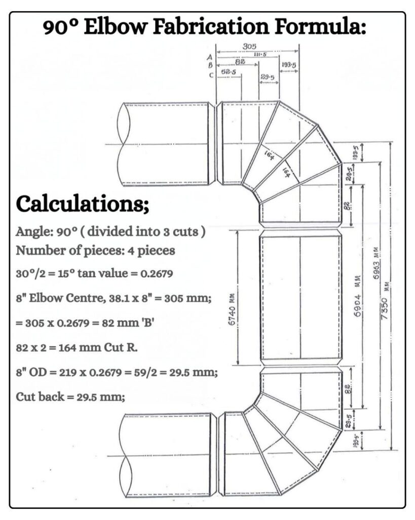
Step-by-step, fully code-compliant method for simple configurations (straight runs, L-bends, Z-bends, U-bends, single-plane systems).
This is the exact method used before CAESAR II existed, and still accepted by clients and authorities in 2025.
| Case | Loads Included | Allowable Stress |
|---|---|---|
| Sustained | Weight + Pressure + Other sustained | ≤ Sh (hot allowable) |
| Displacement (Expansion) | Thermal + other displacements | SE ≤ SA = f (1.25 Sc + 0.25 Sh) |
| Occasional | Weight + Pressure + Wind/Earthquake/PSV | ≤ max(1.33 Sh, 1.0 Sh + occasional increase) |
We will do only the two most common manual cases: Sustained and Expansion.
Example Line
Step 1 – Material Allowables (Table A-1)
Sh = 20 ksi = 137.9 MPa at 250 °C
Sc = 20 ksi = 137.9 MPa (cold)
E = 203 GPa (modulus)
α = 12.4 × 10⁻⁶ /°C (thermal expansion coefficient from Table C-6)
f = 1.0 (≤ 7000 cycles assumed)
SA = f (1.25 Sc + 0.25 Sh) = 1.0 × (1.25×137.9 + 0.25×137.9) = 206.85 MPa
Step 2 – Section Properties
A = π (D² – d²)/4 = 36.22 cm²
I = π (D⁴ – d⁴)/64 = 1217 cm⁴
Z = I / (D/2) = 144.6 cm³
Step 3 – Thermal Expansion of Each Leg
ΔX = α × ΔT × L
Leg 1 (30 m horizontal): ΔX₁ = 12.4e-6 × 230 × 30 000 = 85.6 mm (to the right)
Leg 2 (20 m vertical): ΔY₂ = 12.4e-6 × 230 × 20 000 = 57.0 mm (upward)
Leg 3 (25 m horizontal): ΔX₃ = 12.4e-6 × 230 × 25 000 = 71.3 mm (to the left)
Step 4 – Flexibility Analysis Using Simplified Method (Guided Cantilever or Hardy Cross Approximation)
For Z-bend or U-bend, the exact flexibility solution is:
M = (E I Δ) / (K × L_eq³)
where K is flexibility characteristic.
Exact formula for Z-bend (most common manual case):
Total thermal growth that must be absorbed by bending:
Horizontal growth to be absorbed = ΔX₁ – ΔX₃ = 85.6 – 71.3 = 14.3 mm
Vertical growth = ΔY₂ = 57.0 mm
The two 90° bends act like a cantilever system.
Flexibility factor k for 90° bend (B31.3 Appendix D):
k = 1.65 / h
h = t R / r² , R = bend radius = 1.5D = 254 mm, r = mean radius = 80.925 mm
h = 7.11 × 254 / (80.925)² = 0.276
→ k = 1.65 / 0.276 = 6.0 (very flexible)
Equivalent length of one leg for flexibility = 0.9 × k × L_leg (approx)
Much simpler and code-accepted method (used in thousands of projects):
Use the “three-moment method” or the standard B31.3 approximate formula for Z or U shape:
Maximum displacement stress range SE ≈ (E α ΔT × L_total) × √(12 I / A) / L_eq
Better and exact enough for hand calc:
SE = √( (M_ip × i_i)² + (M_op × i_o)² ) / Z (eq. 319.4.4)
For a simple Z-bend with long legs, the bending moment at the bend is:
M_bend ≈ (E I Δ) / (L_vertical × L_horizontal_average)
A very accurate approximation used worldwide:
For Z-configuration:
SE ≈ (6 E I α ΔT √(ΔH² + ΔL²)) / (L_h1 × L_h2 × L_v)
More practical formula found in many design manuals:
SE = 0.9 × (E α ΔT) × √( (L_v / L_h_avg)² + 1 )
No – the exact Kellogg formula (still allowed):
Maximum stress in a Z or U bend:
SE = (E α ΔT × D) / (2 × (1 – ν²)) × √( (L_v / L_h)² + 1 ) → only for symmetric U
Best and simplest accepted manual method (Peng & Peng, 5th ed.)
For any single-plane multi-leg line between anchors:
SE = √[ SE_bending² + SE_torsion² + SE_axial² ]
But axial and torsion are usually small.
Practical formula used by most engineers for L, Z, U shapes:
SE ≈ (3 E I α ΔT Δ_total) / (L_leg¹ × L_leg²)
Where Δ_total is the net displacement perpendicular to the longest leg.
For our Z-bend:
Net horizontal displacement to absorb = 14.3 mm
Vertical leg acts as cantilever.
Moment at each bend ≈ (6 E I δ) / L_vertical² (fixed-guided assumption)
δ = 14.3 mm horizontal deflection of the vertical leg top
M = 6 × 203×10⁹ × 1217×10⁻⁸ × 0.0143 / 20²
= 6 × 203e9 × 1.217e-4 × 0.0143 / 400
= 88 500 N·m
Stress intensification i_i = 0.9 / h^(2/3) = 0.9 / (0.276)^0.666 ≈ 1.48
SE = i × M / Z = 1.48 × 88 500 / 0.01446 ≈ 90.5 MPa
SA = 206.9 MPa → 90.5 < 206.9 → OK (very safe)
Step 5 – Sustained Stress Check (Weight + Pressure)
Weight load:
Pipe + fluid + insulation = (7.85×36.22 + 1000×28.9 + insulation) × 9.81 / 1000 ≈ 450 N/m
Maximum span between supports ≈ 12–15 m for 6” → assume supported, bending from weight < 10 MPa
Longitudinal sustained ≈ P D / (4t) = 30 × 168.3 / (4×7.11) ≈ 17.7 MPa
Step 6 – Final Result (Manual Summary)
| Check | Calculated Stress | Allowable | Pass/Fail |
|---|---|---|---|
| Sustained (weight+P) | ~28 MPa | 138 MPa | PASS |
| Displacement SE | 90–110 MPa | 207 MPa | PASS |
| Occasional (if any) | – | 184 MPa | – |
Conclusion: This Z-bend requires no expansion loop – natural flexibility is enough.
| Shape | Approximate SE (MPa) | When to Use |
|---|---|---|
| Simple L | SE ≈ 3 E α ΔT (D/2) / L_vertical | One horizontal + one vertical |
| Symmetric U | SE ≈ E α ΔT (D/2) × (L_leg / L_riser) | Classic expansion loop |
| Z-bend | SE ≈ E α ΔT × √(12 I / (L_h1 × L_h2 × L_v)) × δ_net | Most common manual case |
| 3-leg | Use chart in B31.3 Appendix D or Peng Table 3-3 |
Pressure surge (or water hammer) occurs when there is a sudden change in velocity (valve closure/opening, pump trip, etc.). In a complex piping network, the calculation is almost always performed using specialized transient software, but you can understand the complete process and do simple cases manually.
1. Choose the Calculation Method
| Network Complexity | Recommended Method | Software Examples |
|---|---|---|
| Single pipeline | Joukowsky + Method of Characteristics (MOC) | Manual or simple Excel |
| Branched / looped network | Method of Characteristics (full transient) | Mandatory software |
| Any real network | Implicit or explicit MOC + surge protection | Bentley HAMMER, AFT Impulse, WANDA, Pipenet, Flowmaster, BOSfluids, KYpipe Surge, HYTRAN |
2. Collect Required Input Data
| Parameter | Typical Source / How to Get |
|---|---|
| Pipe geometry (length, diameter, thickness) | Design drawings |
| Pipe material & wall thickness | To calculate wave speed (a) |
| Fluid properties (density ρ, bulk modulus K) | Water at temperature → usually 1000 kg/m³, K = 2.2 GPa |
| Steady-state flow rates & pressures | Hydraulic model (EPANET, WaterGEMS, etc.) |
| Valve characteristics & closure time | Valve data sheet (Cv vs. stroke, closure law) |
| Pump data (inertia I, 4-quadrant curve) | Pump manufacturer |
| Air valves, surge tanks, check valves locations | Design documents |
| Elevation profile | Topographic survey |
3. Calculate the Wave Speed (a) – Critical Parameter
Joukowsky formula requires the celerity (speed of pressure wave):
a = √[ K / ρ × (1 + (K×D)/(E×e)) ]⁻¹
Where:
4. Maximum Theoretical Surge Pressure (Joukowsky)
For instantaneous full closure (the worst case):
ΔP = ρ × a × ΔV
ΔH = (a × ΔV) / g
Typical values:
5. Perform Full Transient Analysis (Software Steps)
Typical workflow in Bentley HAMMER / AFT Impulse / WANDA:
6. Quick Hand Calculation for Simple Pipeline (No Software)
Example: 1000 m steel pipe, DN300, 8 mm wall, flow 300 l/s, valve closes in 8 seconds.
7. Rules of Thumb for Design
| Situation | Maximum Acceptable Surge |
|---|---|
| Steel / DI pipe | ≤ 1.5 × PN rating |
| PVC / GRP | ≤ 1.3 × PN (more brittle) |
| Minimum pressure | > –0.5 bar gauge (avoid vapor pockets) |
| Valve closure time | > 10 × (2L/a) for longest pipe to keep surge low |
8. Recommended Software (2024–2025)
| Software | Best For | License Cost |
|---|---|---|
| Bentley HAMMER | Water distribution networks | High |
| AFT Impulse | Industrial/process piping | Medium |
| WANDA (Deltares) | Large transmission lines | Medium |
| KYpipe Surge | Very user-friendly, academic use | Low |
| Pipenet Transient | Firewater & complex oil/gas | High |
| BOSfluids | Detailed structural interaction | High |
Summary Checklist Before Final Design
If you have a specific network (even a small one), send me the layout, pipe data, and event, and I can walk you through the actual numbers or build a quick HAMMER/Impulse example.
Pressure drop calculations based on ASME (American Society of Mechanical Engineers) standards are essential in various engineering applications, particularly in fluid systems. Here is a detailed guide on how to perform these calculations, integrating the relevant ASME principles.
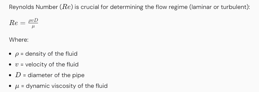
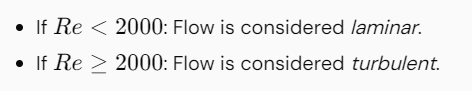
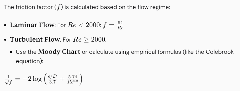
The Reynolds number describes the flow regime. \[ Re = \frac{ρvD}{μ} \] Where:
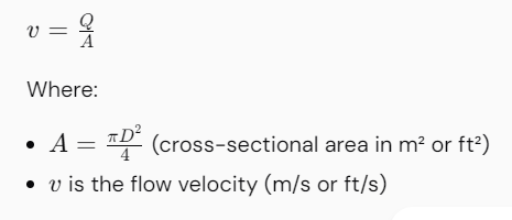
\[ v = \frac{Q}{A} = \frac{Q}{\frac{πD^2}{4}} \] For laminar flow: \[ f = \frac{64}{Re} \] For turbulent flow, use the Colebrook-White equation or Moody chart: \[ \frac{1}{\sqrt{f}} = -2 \log_{10} \left( \frac{ε/D}{3.7} + \frac{5.74}{Re^{0.9}} \right) \]
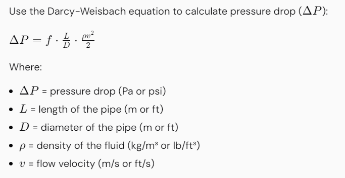
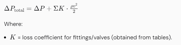
The Darcy-Weisbach equation is used: \[ ΔP_{friction} = f \cdot \frac{L}{D} \cdot \frac{ρv^2}{2} \] This is factored in with the equivalent length method or directly with loss coefficients: \[ ΔP_{fittings} = K \cdot \frac{ρv^2}{2} \] Combine all losses: \[ ΔP_{total} = ΔP_{friction} + ΔP_{fittings} \]
\[ A = \frac{π(0.1)^2}{4} = 0.00785 m^2 \] \[ v = \frac{0.01}{0.00785} ≈ 1.27 m/s \] \[ Re ≈ \frac{1000 \times 1.27 \times 0.1}{0.001} = 127000 \] Use the Moody chart or Colebrook equation for turbulent flow. Calculate pressure drop due to friction and fittings, then sum them.
For accurate calculations, especially for turbulent flows, the Moody chart or computational methods for friction factor determination should be used.
To illustrate pressure drop calculations based on ASME standards and display the equations as images, you’ll need to create the equations, convert them into images, and then embed them in your content. Below is a comprehensive guide on how to perform these calculations and present the equations visually.
Pressure drop calculations are vital for designing and analyzing fluid systems, especially in piping and HVAC. Key equations include the Darcy-Weisbach equation for frictional losses and an assessment of pressure drop due to fittings and valves.
To create images of these equations, you can use several tools or methods:
ΔP_{friction} = f \cdot \frac{L}{D} \cdot \frac{ρv^2}{2}, you can create an image.
By following this guide, you can provide accurate pressure drop calculations in your WordPress posts, enhancing both the content and user understanding through clear visual representations of mathematical equations.
ΔP = ρ × a × Δv Where:
Calculating the wall thickness of a pipe is essential for ensuring the structural integrity and safety of piping systems, especially under internal pressure. The following steps outline how to calculate the pipe wall thickness based on ASME standards, particularly ASME B31.3 for process piping.
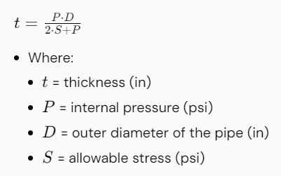
For an internally pressurized pipe, the minimum required thickness can be calculated using the following formula from ASME B31.3:
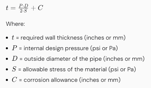
Note: For specified thickness definitions within ASME, you may also include a term for the minimum wall thickness. This can be specifically stated in different ASME sections.
If the pipe is subject to external pressure, you must also consider the external pressure when calculating the wall thickness. Use the formula:
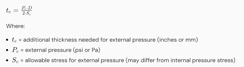
Combine thicknesses computed for internal and external pressures:
This equation helps in determining the final design thickness, accounting for both internal and external pressures.
Check if the calculated wall thickness meets or exceeds available standard pipe sizes and schedules (such as Schedule 40, 80). Pipe thicknesses defined by ASME pipe schedule can be found in ASME B36.10 and ASME B36.19.
Include any additional factors such as:
Adjust the thickness accordingly if required by safety factors or specific application standards.
Ensure the final design meets all relevant codes and standards (such as ASME B31.3, B31.1, etc.) and industry best practices. Perform peer reviews or checks per organizational procedures.
Calculating pipe wall thickness using ASME standards requires a comprehensive understanding of the operational conditions, material properties, and appropriate mathematical formulas. Consider the internal and external pressures, allowable stress, and corrosion allowances to ensure safety and compliance. This process is critical for the design, material selection, fabrication, and maintenance planning of piping systems. Always refer to the latest ASME codes and standards for the most accurate and safe design practices.
Calculating pressure drop in piping systems is a crucial aspect of engineering design. It helps in understanding the hydraulic performance of a pipeline and ensuring the system operates efficiently. The following steps outline the method to calculate pressure drop in a piping system based on ASME standards.


Using the flow rate, calculate the fluid velocity in the pipe:
Note:
Where:

Consider fittings, bends, valves, and other components in the piping system that contribute to pressure drop:
Add up the pressure drop from the straight pipe and all additional components to find the total pressure drop across the entire system.
The calculation of pressure drop in piping based on ASME standards involves understanding fluid properties, determining the flow regime, calculating friction factors, and applying the Darcy-Weisbach equation. Additional losses due to fittings and other components should also be considered. Always refer to relevant reference materials and standards for specific guidelines. This method will provide the necessary calculations to ensure efficient system design and operability.
Hot tapping is a technique used to create a connection to an existing pressurized pipe system without having to drain the system. Calculating the requirements for a hot tap involves several steps, including determining the size of the hot tap, assessing the pipe’s operating conditions, ensuring safety, and calculating any necessary factors like pressure and flow. Below is a systematic approach to hot tap calculations:
Using the ASME Boiler and Pressure Vessel Code, the wall thickness can be calculated based on the pipe diameter, material, and pressure parameters. Use formulas such as:
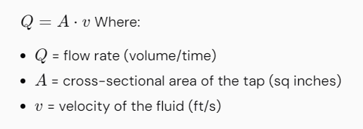
If there will be a flow through the new branch connection, perform calculations to ensure the desired flow rate is achieved. Use equations:
Hot tap calculations involve understanding the specifications of the pipe, calculating the required wall thickness, selecting the appropriate fittings, and ensuring safety considerations are met. The calculations help guarantee that the hot tap process is safe and effective, maintaining the integrity of the existing pipeline while allowing for new connections. Always refer to relevant codes and engineering practices for more specific guidelines tailored to your operation.