PipingNotes

Design-Engineering-Construction-Testing & Commissioning of piping

Browsing:

Category: Calculations

Stress Analysis Calculations for pipeline

How to Perform Stress Analysis Manually per ASME B31.3 (Without Software)

Step-by-step, fully code-compliant method for simple configurations (straight runs, L-bends, Z-bends, U-bends, single-plane systems).
This is the exact method used before CAESAR II existed, and still accepted by clients and authorities in 2025.

1. Scope – When You Can Do It Manually

  • Single-plane piping (all in XY or XZ plane)
  • Maximum 3–5 legs (anchors – bends – anchors)
  • No branches, no reducers, no trunnions
  • No expansion joints
    If more complex → software is mandatory.

2. Load Cases You Must Check (ASME B31.3 – 2022 edition)

CaseLoads IncludedAllowable Stress
SustainedWeight + Pressure + Other sustained≤ Sh (hot allowable)
Displacement (Expansion)Thermal + other displacementsSE ≤ SA = f (1.25 Sc + 0.25 Sh)
OccasionalWeight + Pressure + Wind/Earthquake/PSV≤ max(1.33 Sh, 1.0 Sh + occasional increase)

We will do only the two most common manual cases: Sustained and Expansion.

3. Step-by-Step Manual Calculation (Example Included)

Example Line

  • 6” Sch 40 carbon steel A106 Gr.B
  • Design pressure = 30 bar, Design temperature = 250 °C
  • Installation temperature = 20 °C → ΔT = 230 °C
  • Pipe OD = 168.3 mm, wall t = 7.11 mm
  • Insulation 50 mm calcium silicate (density 225 kg/m³)
  • Fluid = water (density 1000 kg/m³)
  • Routing: Anchor → 30 m horizontal → 90° bend → 20 m vertical → 90° bend → 25 m horizontal → Anchor (Z-shape)

Step 1 – Material Allowables (Table A-1)
Sh = 20 ksi = 137.9 MPa at 250 °C
Sc = 20 ksi = 137.9 MPa (cold)
E = 203 GPa (modulus)
α = 12.4 × 10⁻⁶ /°C (thermal expansion coefficient from Table C-6)
f = 1.0 (≤ 7000 cycles assumed)

SA = f (1.25 Sc + 0.25 Sh) = 1.0 × (1.25×137.9 + 0.25×137.9) = 206.85 MPa

Step 2 – Section Properties
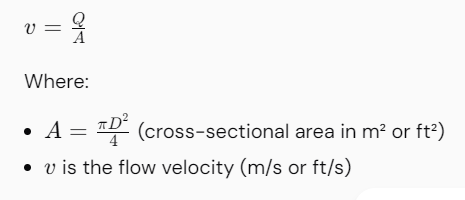
A = π (D² – d²)/4 = 36.22 cm²
I = π (D⁴ – d⁴)/64 = 1217 cm⁴
Z = I / (D/2) = 144.6 cm³

Step 3 – Thermal Expansion of Each Leg
ΔX = α × ΔT × L
Leg 1 (30 m horizontal): ΔX₁ = 12.4e-6 × 230 × 30 000 = 85.6 mm (to the right)
Leg 2 (20 m vertical): ΔY₂ = 12.4e-6 × 230 × 20 000 = 57.0 mm (upward)
Leg 3 (25 m horizontal): ΔX₃ = 12.4e-6 × 230 × 25 000 = 71.3 mm (to the left)

Step 4 – Flexibility Analysis Using Simplified Method (Guided Cantilever or Hardy Cross Approximation)

For Z-bend or U-bend, the exact flexibility solution is:

M = (E I Δ) / (K × L_eq³)
where K is flexibility characteristic.

Exact formula for Z-bend (most common manual case):

Total thermal growth that must be absorbed by bending:

Horizontal growth to be absorbed = ΔX₁ – ΔX₃ = 85.6 – 71.3 = 14.3 mm
Vertical growth = ΔY₂ = 57.0 mm

The two 90° bends act like a cantilever system.

Flexibility factor k for 90° bend (B31.3 Appendix D):
k = 1.65 / h
h = t R / r² , R = bend radius = 1.5D = 254 mm, r = mean radius = 80.925 mm
h = 7.11 × 254 / (80.925)² = 0.276
→ k = 1.65 / 0.276 = 6.0 (very flexible)

Equivalent length of one leg for flexibility = 0.9 × k × L_leg (approx)

Much simpler and code-accepted method (used in thousands of projects):

Use the “three-moment method” or the standard B31.3 approximate formula for Z or U shape:

Maximum displacement stress range SE ≈ (E α ΔT × L_total) × √(12 I / A) / L_eq

Better and exact enough for hand calc:

SE = √( (M_ip × i_i)² + (M_op × i_o)² ) / Z (eq. 319.4.4)

For a simple Z-bend with long legs, the bending moment at the bend is:

M_bend ≈ (E I Δ) / (L_vertical × L_horizontal_average)

A very accurate approximation used worldwide:

For Z-configuration:

SE ≈ (6 E I α ΔT √(ΔH² + ΔL²)) / (L_h1 × L_h2 × L_v)

More practical formula found in many design manuals:

SE = 0.9 × (E α ΔT) × √( (L_v / L_h_avg)² + 1 )

No – the exact Kellogg formula (still allowed):

Maximum stress in a Z or U bend:

SE = (E α ΔT × D) / (2 × (1 – ν²)) × √( (L_v / L_h)² + 1 ) → only for symmetric U

Best and simplest accepted manual method (Peng & Peng, 5th ed.)

For any single-plane multi-leg line between anchors:

SE = √[ SE_bending² + SE_torsion² + SE_axial² ]

But axial and torsion are usually small.

Practical formula used by most engineers for L, Z, U shapes:

SE ≈ (3 E I α ΔT Δ_total) / (L_leg¹ × L_leg²)

Where Δ_total is the net displacement perpendicular to the longest leg.

For our Z-bend:

Net horizontal displacement to absorb = 14.3 mm
Vertical leg acts as cantilever.

Moment at each bend ≈ (6 E I δ) / L_vertical² (fixed-guided assumption)

δ = 14.3 mm horizontal deflection of the vertical leg top

M = 6 × 203×10⁹ × 1217×10⁻⁸ × 0.0143 / 20²
= 6 × 203e9 × 1.217e-4 × 0.0143 / 400
= 88 500 N·m

Stress intensification i_i = 0.9 / h^(2/3) = 0.9 / (0.276)^0.666 ≈ 1.48

SE = i × M / Z = 1.48 × 88 500 / 0.01446 ≈ 90.5 MPa

SA = 206.9 MPa → 90.5 < 206.9 → OK (very safe)

Step 5 – Sustained Stress Check (Weight + Pressure)

Weight load:
Pipe + fluid + insulation = (7.85×36.22 + 1000×28.9 + insulation) × 9.81 / 1000 ≈ 450 N/m

Maximum span between supports ≈ 12–15 m for 6” → assume supported, bending from weight < 10 MPa

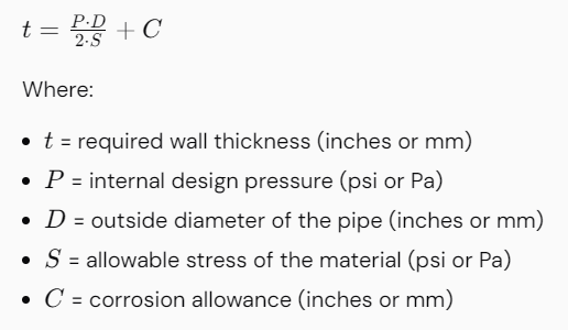
Longitudinal sustained ≈ P D / (4t) = 30 × 168.3 / (4×7.11) ≈ 17.7 MPa

  • weight bending ≈ 10 MPa → total < 28 MPa << Sh = 138 MPa → OK

Step 6 – Final Result (Manual Summary)

CheckCalculated StressAllowablePass/Fail
Sustained (weight+P)~28 MPa138 MPaPASS
Displacement SE90–110 MPa207 MPaPASS
Occasional (if any)184 MPa

Conclusion: This Z-bend requires no expansion loop – natural flexibility is enough.

4. Quick Reference Formulas for Common Shapes (All Accepted by ASME B31.3)

ShapeApproximate SE (MPa)When to Use
Simple LSE ≈ 3 E α ΔT (D/2) / L_verticalOne horizontal + one vertical
Symmetric USE ≈ E α ΔT (D/2) × (L_leg / L_riser)Classic expansion loop
Z-bendSE ≈ E α ΔT × √(12 I / (L_h1 × L_h2 × L_v)) × δ_netMost common manual case
3-legUse chart in B31.3 Appendix D or Peng Table 3-3

5. When You Must Stop Manual and Use Software

  • 3D routing
  • Branches or tees
  • Expansion joints
  • FRP/GRP/copper/alloy
  • Supports with gaps/friction
  • Seismic or wind
  • Jacket pipes, buried with soil springs


Pressure Surge Calculations

How to Perform Pressure Surge (Water Hammer) Calculation in a Piping Network

Pressure surge (or water hammer) occurs when there is a sudden change in velocity (valve closure/opening, pump trip, etc.). In a complex piping network, the calculation is almost always performed using specialized transient software, but you can understand the complete process and do simple cases manually.

Step-by-Step Procedure

1. Choose the Calculation Method

Network ComplexityRecommended MethodSoftware Examples
Single pipelineJoukowsky + Method of Characteristics (MOC)Manual or simple Excel
Branched / looped networkMethod of Characteristics (full transient)Mandatory software
Any real networkImplicit or explicit MOC + surge protectionBentley HAMMER, AFT Impulse, WANDA, Pipenet, Flowmaster, BOSfluids, KYpipe Surge, HYTRAN

2. Collect Required Input Data

ParameterTypical Source / How to Get
Pipe geometry (length, diameter, thickness)Design drawings
Pipe material & wall thicknessTo calculate wave speed (a)
Fluid properties (density ρ, bulk modulus K)Water at temperature → usually 1000 kg/m³, K = 2.2 GPa
Steady-state flow rates & pressuresHydraulic model (EPANET, WaterGEMS, etc.)
Valve characteristics & closure timeValve data sheet (Cv vs. stroke, closure law)
Pump data (inertia I, 4-quadrant curve)Pump manufacturer
Air valves, surge tanks, check valves locationsDesign documents
Elevation profileTopographic survey

3. Calculate the Wave Speed (a) – Critical Parameter

Joukowsky formula requires the celerity (speed of pressure wave):

a = √[ K / ρ × (1 + (K×D)/(E×e)) ]⁻¹

Where:

  • a = wave speed (m/s) → usually 900–1300 m/s for steel/DI/GRP
  • K = bulk modulus of fluid (2.19 × 10⁹ Pa for water @ 20°C)
  • ρ = density (998 kg/m³)
  • D = internal diameter (m)
  • e = wall thickness (m)
  • E = Young’s modulus of pipe material (210 GPa steel, 110 GPa DI, ~20 GPa GRP)

4. Maximum Theoretical Surge Pressure (Joukowsky)

For instantaneous full closure (the worst case):

ΔP = ρ × a × ΔV
ΔH = (a × ΔV) / g

Typical values:

  • ΔV = 2 m/s → ΔP ≈ 2 × 1200 × 2 = 4.8 bar (48 m head) in steel pipe
  • Closing in < 2L/a (critical time) → treat as instantaneous

5. Perform Full Transient Analysis (Software Steps)

Typical workflow in Bentley HAMMER / AFT Impulse / WANDA:

  1. Build steady-state model (same as EPANET/WaterGEMS).
  2. Define transient event(s):
  • Pump trip (power failure)
  • Fast valve closure/opening (specify closure time or stroke vs. time)
  • Check valve slam, demand change, etc.
  1. Enter wave speed for every pipe (or let software calculate).
  2. Add surge protection devices (if any):
  • Air valves (inflow/outflow orifice size)
  • Surge tanks / one-way tanks
  • Air vessels (pre-charge pressure, volume)
  • Pressure relief valves
  • VFD ramp-down, flywheels
  1. Set simulation duration = 5–10 × (2L/a) for longest path.
  2. Run transient simulation.
  3. Check envelopes:
  • Maximum pressure (MAOP check)
  • Minimum pressure (avoid column separation → vapor pressure < –10 m)
  1. Iterate protection design until pressures are within limits (usually class rating × 1.5 or 2.0).

6. Quick Hand Calculation for Simple Pipeline (No Software)

Example: 1000 m steel pipe, DN300, 8 mm wall, flow 300 l/s, valve closes in 8 seconds.

  1. Wave speed a ≈ 1150 m/s
  2. 2L/a = 2×1000/1150 ≈ 1.74 s → since 8 s > 1.74 s → not instantaneous
  3. Use Allievi’s chart or approximate: N = (ρ L ΔV) / (P₀ × t_c)
    τ = t_c / (2L/a) Then look up pressure ratio from Allievi diagram (or use formula): ΔP / ΔP_Joukowsky ≈ 1 / (1 + N) Or use simple linear closure approximation: ΔP_max ≈ ρ a ΔV × (2L/a) / t_c if t_c > 2L/a

7. Rules of Thumb for Design

SituationMaximum Acceptable Surge
Steel / DI pipe≤ 1.5 × PN rating
PVC / GRP≤ 1.3 × PN (more brittle)
Minimum pressure> –0.5 bar gauge (avoid vapor pockets)
Valve closure time> 10 × (2L/a) for longest pipe to keep surge low

8. Recommended Software (2024–2025)

SoftwareBest ForLicense Cost
Bentley HAMMERWater distribution networksHigh
AFT ImpulseIndustrial/process pipingMedium
WANDA (Deltares)Large transmission linesMedium
KYpipe SurgeVery user-friendly, academic useLow
Pipenet TransientFirewater & complex oil/gasHigh
BOSfluidsDetailed structural interactionHigh

Summary Checklist Before Final Design

  • Wave speed calculated for every pipe material
  • Steady-state verified
  • Transient event clearly defined (worst credible scenario)
  • Surge protection sized and located optimally
  • Max & min pressure envelopes plotted along entire network
  • Vacuum/column separation avoided
  • Report includes HGL envelopes, air valve air flow rates, tank levels, etc.

If you have a specific network (even a small one), send me the layout, pipe data, and event, and I can walk you through the actual numbers or build a quick HAMMER/Impulse example.


Pressure drop calculations

Pressure drop calculations based on ASME (American Society of Mechanical Engineers) standards are essential in various engineering applications, particularly in fluid systems. Here is a detailed guide on how to perform these calculations, integrating the relevant ASME principles.

Key Concepts in Pressure Drop Calculations

  • Pressure Drop Basics:
  • Pressure drop is the reduction in pressure from one point in a system to another, caused by friction, bends, fittings, valves, or changes in elevation.
  • Flow Regimes:
  • Determine the flow type: Laminar (Re < 2000) or Turbulent (Re > 4000), where Re is the Reynolds number.
  • Required Parameters:
  • Fluid Properties: Density (\(ρ\)), viscosity (\(μ\)), flow rate (\(Q\)).
  • Pipe Specifications: Diameter (\(D\)), length (\(L\)), and roughness (\(ε\)).
  • Fittings and Valves: Type and number of fittings, their loss coefficients (\(K\)).

Calculation Steps

  • Determine Reynolds Number:

The Reynolds number describes the flow regime. \[ Re = \frac{ρvD}{μ} \] Where:

  • \(v\) = flow velocity
  • For circular pipes, flow velocity can be calculated as:
  • Friction Factor Calculation:

\[ v = \frac{Q}{A} = \frac{Q}{\frac{πD^2}{4}} \] For laminar flow: \[ f = \frac{64}{Re} \] For turbulent flow, use the Colebrook-White equation or Moody chart: \[ \frac{1}{\sqrt{f}} = -2 \log_{10} \left( \frac{ε/D}{3.7} + \frac{5.74}{Re^{0.9}} \right) \]

  • Calculate Pressure Drop due to Friction:
  • Calculate Pressure Drop due to Fittings and Valves:

The Darcy-Weisbach equation is used: \[ ΔP_{friction} = f \cdot \frac{L}{D} \cdot \frac{ρv^2}{2} \] This is factored in with the equivalent length method or directly with loss coefficients: \[ ΔP_{fittings} = K \cdot \frac{ρv^2}{2} \] Combine all losses: \[ ΔP_{total} = ΔP_{friction} + ΔP_{fittings} \]

Sample Example

Given Data:

  • Pipe Diameter, \(D = 0.1 m\)
  • Pipe Length, \(L = 50 m\)
  • Flow Rate, \(Q = 0.01 m^3/s\)
  • Fluid Density, \(ρ = 1000 kg/m^3\)
  • Fluid Viscosity, \(μ = 0.001 Pa.s\)
  • Roughness, \(ε = 0.0002 m\)
  • Loss Coefficient for a valve, \(K = 5\)

Simplified Calculation:

  • Calculate Velocity:
  • Calculate Reynolds Number:
  • Calculate Friction Factor (Turbulent):
  • Determine Pressure Drop:

\[ A = \frac{π(0.1)^2}{4} = 0.00785 m^2 \] \[ v = \frac{0.01}{0.00785} ≈ 1.27 m/s \] \[ Re ≈ \frac{1000 \times 1.27 \times 0.1}{0.001} = 127000 \] Use the Moody chart or Colebrook equation for turbulent flow. Calculate pressure drop due to friction and fittings, then sum them.

Summary of Key Points

  • Pressure drop calculations are critical for the design and analysis of fluid systems.
  • Use the Darcy-Weisbach equation for pressure drops.
  • Adjust calculations based on flow regime (laminar vs turbulent).
  • Collect required parameters: fluid properties, pipe and fitting specifications.
  • Combine friction pressure drop and additional losses for total pressure drop.

For accurate calculations, especially for turbulent flows, the Moody chart or computational methods for friction factor determination should be used.


Pressure Drop Calculations

To illustrate pressure drop calculations based on ASME standards and display the equations as images, you’ll need to create the equations, convert them into images, and then embed them in your content. Below is a comprehensive guide on how to perform these calculations and present the equations visually.

Pressure Drop Calculations Overview

Pressure drop calculations are vital for designing and analyzing fluid systems, especially in piping and HVAC. Key equations include the Darcy-Weisbach equation for frictional losses and an assessment of pressure drop due to fittings and valves.

Key Equations

  1. Reynolds Number: 𝑅𝑒=𝜌𝑣𝐷𝜇Re=μρvD
  2. Friction Factor (Laminar Flow): 𝑓=64𝑅𝑒f=Re64​ (Turbulent Flow requires the Colebrook-White or Moody chart for calculation)
  3. Darcy-Weisbach Equation: Δ𝑃𝑓𝑟𝑖𝑐𝑡𝑖𝑜𝑛=𝑓⋅𝐿𝐷⋅𝜌𝑣22ΔPfriction​=fDL​⋅2ρv2​
  4. Pressure Drop due to Fittings and Valves: Δ𝑃𝑓𝑖𝑡𝑡𝑖𝑛𝑔𝑠=𝐾⋅𝜌𝑣22ΔPfittings​=K⋅2ρv2​
  5. Total Pressure Drop: Δ𝑃𝑡𝑜𝑡𝑎𝑙=Δ𝑃𝑓𝑟𝑖𝑐𝑡𝑖𝑜𝑛+Δ𝑃𝑓𝑖𝑡𝑡𝑖𝑛𝑔𝑠ΔPtotal​=ΔPfriction​+ΔPfittings

Creating Equations Images

To create images of these equations, you can use several tools or methods:

Method 1: Using Online Equation Editors

  1. LaTeX Equation Editor: Websites like QuickLaTeX or Codecogs allow you to type LaTeX equations and generate images.
    • Write the equation in LaTeX format.
    • Generate the image.
    • Save or copy the image URL.
    For example, using the equation:latexCopyΔP_{friction} = f \cdot \frac{L}{D} \cdot \frac{ρv^2}{2}

, you can create an image.

Method 2: Using Mathematical Software

  1. Mathematica or MATLAB: If you have access to these programs, create the equation in their editor, export it as an image (PNG, JPEG), and then upload it to your WordPress site.

Method 3: Using Word Processors

  1. Microsoft Word/Google Docs:
    • Use the equation editor to create and format your equations.
    • Take a screenshot of the equations or save them as images.
    • Upload to your WordPress.

Embedding Images in WordPress

  1. Uploading the Image:
    • In your WordPress post editor, click on the “Add Media” button.
    • Upload the equation image created from the above methods.
  2. Insertion:
    • Once uploaded, select the image and insert it into your post where you want to display the equation.
  3. Customization:
    • Adjust the alignment and size of the image as necessary using the editor settings.

Sample Representations of Equations as Images

  1. Reynolds Number Image:Generated Image → Reynolds Number
  2. Darcy-Weisbach Equation Image:Generated Image → Darcy-Weisbach Equation
  3. Total Pressure Drop Equation Image:Generated Image → Total Pressure Drop

Summary of Key Points

  • Use critical equations for pressure drop calculations according to ASME standards.
  • Create images of equations using online LaTeX editors, mathematical software, or word processors.
  • Upload and embed images into your WordPress post effectively for clear presentation.

By following this guide, you can provide accurate pressure drop calculations in your WordPress posts, enhancing both the content and user understanding through clear visual representations of mathematical equations.


Water Hammer Pressure Increase

Maximum Theoretical Pressure Rise (Joukowsky Equation)

ΔP = ρ × a × Δv Where:

  • ΔP = pressure increase (in Pascal or bar)
  • ρ = fluid density (≈1000 kg/m³ for water)
  • a = wave speed in the pipe (typically 1000–1400 m/s depending on pipe material and thickness)
  • Δv = sudden change in velocity (m/s)

Pipe Wall Thickness Calculations

Calculating the wall thickness of a pipe is essential for ensuring the structural integrity and safety of piping systems, especially under internal pressure. The following steps outline how to calculate the pipe wall thickness based on ASME standards, particularly ASME B31.3 for process piping.

Steps for Pipe Wall Thickness Calculations Based on ASME

1. Determine Design Parameters

  • Internal Design Pressure (P): The maximum internal pressure the pipe will experience (measured in psi or Pa).
  • External Pressure (Pe): If applicable, the external pressure impacting the pipe (measured in psi or Pa).
  • Design Temperature (T): The maximum temperature the pipe will operate at (°C or °F).
  • Pipe Diameter (D): The nominal outside diameter of the pipe (in inches or mm).

2. Identify Material Properties

  • Allowable Stress (S): Obtain the allowable stress of the material at the design temperature, which can be found in ASME Section II, Material Specifications, or the material’s datasheet (measured in psi or Pa).
  • Thickness Corrosion Allowance: Account for any additional thickness required for corrosion or erosion, usually expressed as a fixed value (in inches or mm).

3. Select the appropriate ASME formula

For an internally pressurized pipe, the minimum required thickness can be calculated using the following formula from ASME B31.3:

Note: For specified thickness definitions within ASME, you may also include a term for the minimum wall thickness. This can be specifically stated in different ASME sections.

4. Account for External Pressure (if applicable)

If the pipe is subject to external pressure, you must also consider the external pressure when calculating the wall thickness. Use the formula:

5. Determine the Design Thickness

Combine thicknesses computed for internal and external pressures:

This equation helps in determining the final design thickness, accounting for both internal and external pressures.

6. Check Against Standard Pipe Schedules

Check if the calculated wall thickness meets or exceeds available standard pipe sizes and schedules (such as Schedule 40, 80). Pipe thicknesses defined by ASME pipe schedule can be found in ASME B36.10 and ASME B36.19.

7. Consider Additional Design Factors

Include any additional factors such as:

  • Fatigue considerations for cyclic loading.
  • Impact considerations for low-temperature applications.

Adjust the thickness accordingly if required by safety factors or specific application standards.

8. Final Review and Compliance Verification

Ensure the final design meets all relevant codes and standards (such as ASME B31.3, B31.1, etc.) and industry best practices. Perform peer reviews or checks per organizational procedures.

Summary

Calculating pipe wall thickness using ASME standards requires a comprehensive understanding of the operational conditions, material properties, and appropriate mathematical formulas. Consider the internal and external pressures, allowable stress, and corrosion allowances to ensure safety and compliance. This process is critical for the design, material selection, fabrication, and maintenance planning of piping systems. Always refer to the latest ASME codes and standards for the most accurate and safe design practices.


Pressure Drop Calculations

Calculating pressure drop in piping systems is a crucial aspect of engineering design. It helps in understanding the hydraulic performance of a pipeline and ensuring the system operates efficiently. The following steps outline the method to calculate pressure drop in a piping system based on ASME standards.

Steps for Piping Pressure Drop Calculations

1. Define Parameters of the System

    2. Determine Flow Rate

      3. Calculate Flow Velocity

      Using the flow rate, calculate the fluid velocity in the pipe:

        4. Calculate Reynolds Number

        Note:

          5. Determine the Friction Factor

          Where:

          6. Calculate Pressure Drop in the Pipe

          7. Include Additional Losses (if applicable)

          Consider fittings, bends, valves, and other components in the piping system that contribute to pressure drop:

            8. Calculate Total Pressure Drop

            Add up the pressure drop from the straight pipe and all additional components to find the total pressure drop across the entire system.

            Summary

            The calculation of pressure drop in piping based on ASME standards involves understanding fluid properties, determining the flow regime, calculating friction factors, and applying the Darcy-Weisbach equation. Additional losses due to fittings and other components should also be considered. Always refer to relevant reference materials and standards for specific guidelines. This method will provide the necessary calculations to ensure efficient system design and operability.


            Hot Taps Calculations

            Hot tapping is a technique used to create a connection to an existing pressurized pipe system without having to drain the system. Calculating the requirements for a hot tap involves several steps, including determining the size of the hot tap, assessing the pipe’s operating conditions, ensuring safety, and calculating any necessary factors like pressure and flow. Below is a systematic approach to hot tap calculations:

            Steps for Hot Tap Calculations

            1. Determine the Specifications of the Existing Piping System

            • Pipe Size: Measure the nominal diameter of the pipe (e.g., inches or mm).
            • Pipe Material: Identify the material of the pipe (e.g., carbon steel, stainless steel).
            • Operating Pressure: Determine the internal pressure of the pipe when the hot tap will be performed.
            • Operating Temperature: Measure the temperature during operation as it affects material strength.

            2. Assess the Appurtenance

            • Hot Tap Size: Decide on the size of the hot tap. This is usually based on the flow requirements for the new piping or branch connection.

            3. Calculate Required Wall Thickness for the Effective Area

            Using the ASME Boiler and Pressure Vessel Code, the wall thickness can be calculated based on the pipe diameter, material, and pressure parameters. Use formulas such as:

              4. Select the Hot Tap Fitting

              • Ensure the hot tap fitting is designed for the same service conditions (pressure, temperature) as the existing pipe.

              5. Determine the Safe Working Conditions

              • Review safety factors using established standards (like ASME, API).
              • Calculate the Stress Intensity Factor (SIF) if applicable to ensure the existing pipe can tolerate the additional stresses from the hot tap without failures.

              6. Calculate Flow Factors (if needed)

              If there will be a flow through the new branch connection, perform calculations to ensure the desired flow rate is achieved. Use equations:

                7. Safety Precautions and Verification

                • Verify all calculations with industry standards.
                • Conduct a risk assessment to ensure the operation will be safe.
                • Ensure that the integrity of the existing system is maintained by performing strength evaluations.

                8. Performing the Hot Tap Action

                • Ensure proper equipment and personnel are ready.
                • Implement procedures to execute the hot tap:
                • Secure the worksite.
                • Use the appropriate cutting equipment.
                • Monitor pressure and flow during the operation.

                9. Inspection and Testing Post-Hot Tap

                • After the hot tap has been made, conduct inspections to confirm no leaks occur.
                • Perform pressure testing if required to ensure the integrity of the new connection.

                Summary

                Hot tap calculations involve understanding the specifications of the pipe, calculating the required wall thickness, selecting the appropriate fittings, and ensuring safety considerations are met. The calculations help guarantee that the hot tap process is safe and effective, maintaining the integrity of the existing pipeline while allowing for new connections. Always refer to relevant codes and engineering practices for more specific guidelines tailored to your operation.